
 Q. No.
A cell having an emf \(\varepsilon\) and internal resistance \(r\) is connected across a variable external resistance \(R\). As the resistance \(R\) is increased, the plot of potential difference \(V\) across \(R\) is given by:
1.

2.

3.

4.


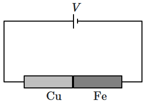
In the circuit shown in the figure below, if the potential at point \(A\) is taken to be zero, the potential at point \(B\) will be:

1. \(+1\) V
2. \(-1\) V
3. \(+2\) V
4. \(-2\) V
A thermocouple of negligible resistance produces an e.m.f. of 40 µV/ºC in the linear range of temperature. A galvanometer of resistance 10 ohm whose sensitivity is 1 µA/division, is employed with the thermocouple. The smallest value of temperature difference that can be detected by the system will be:
1. 0.25ºC
2. 0.5 ºC
3. 1ºC
4. 0.1ºC


The thermo e.m.f E in volts of a certain thermocouple is found to vary with temperature difference θ in ºC between the two junctions according to the relation
The neutral temperature for the thermo-couple will be:
1. 400ºC
2. 225ºC
3. 30ºC
4. 450ºC
The power dissipated in the circuit shown in the figure is \(30~\text{Watts}\). The value of \(R\) is:
1. \(15~\Omega\)
2. \(10~\Omega\)
3. \(30~\Omega\)
4. \(20~\Omega\)

| 1. | \(0.00145~\text V\) | 2. | \(0.0145~\text V\) |
| 3. | \(1.7\times10^{-6}~\text V\) | 4. | \(0.117~\text V\) |


1. \(9:16:25\)
2. \(27:32:35\)
3. \(21:24:25\)
4. \(3:4:5\)
| 1. | \(20\) | 2. | \(30\) |
| 3. | \(40\) | 4. | \(10\) |
Kirchhoff’s first and second laws for electrical circuits are consequences of:
| 1. | conservation of energy. |
| 2. | conservation of electric charge and energy respectively. |
| 3. | conservation of electric charge. |
| 4. | conservation of energy and electric charge respectively. |


The power dissipated across the \(8~\Omega\) resistor in the circuit shown here is \(2~\text{W}\). The power dissipated in watts across the \(3~\Omega\) resistor is:

| 1. | \(2.0\) | 2. | \(1.0\) |
| 3. | \(0.5\) | 4. | \(3.0\) |
© 2026 GoodEd Technologies Pvt. Ltd.